Chapter 16 — Probability: Theoretical and Experimental

Standard: 7.PS.1 — The student will use statistical investigation to determine the probability of an event and investigate and describe the difference between the experimental and theoretical probability.

By the end of this chapter you will be able to:

• Determine the theoretical probability of an event by counting the outcomes in a sample space (7.PS.1a)
• Given the results of a statistical investigation, determine the experimental probability of an event (7.PS.1b)
• Describe how the experimental probability changes as the number of trials increases (7.PS.1c)
• Investigate and describe the difference between the probability of an event found through experiment or simulation and the theoretical probability of that same event (7.PS.1d)

Lessons: 16.1 Theoretical Probability · 16.2 Experimental Probability · 16.3 What Happens as the Number of Trials Grows · 16.4 Comparing Theoretical and Experimental Probability

Every other chapter in this book has asked you to find a number that is exactly right. This one asks something different. Probability does not tell you what will happen on the next roll of a die — nothing can. It tells you what to expect in the long run, and how much the short run is allowed to wander away from that expectation. You will spend this chapter doing two kinds of work side by side: reasoning about what should happen, and gathering real data about what did happen. Learning how those two numbers relate — and how they fail to relate — is the point.

Lesson 16.1 — Theoretical Probability

Outcomes, sample spaces, and events

A probability experiment is any action with a result you cannot predict with certainty: flipping a coin, rolling a die, spinning a spinner, drawing a marble from a bag without looking.

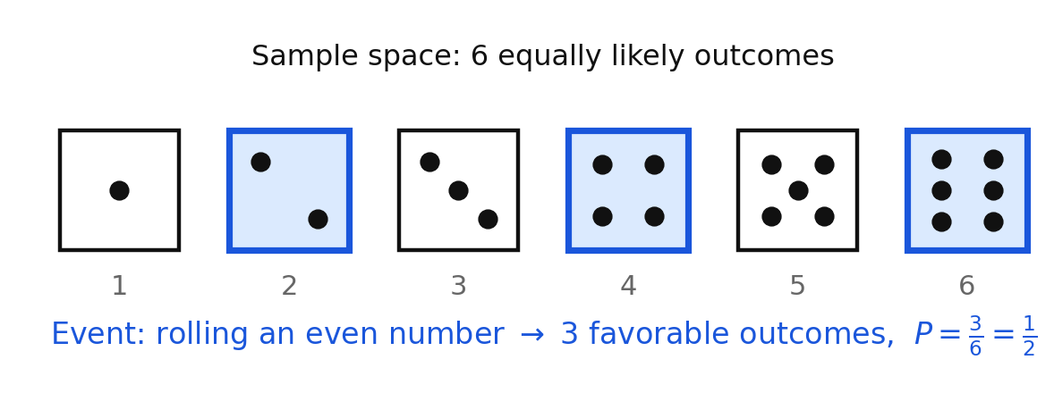
Each single possible result is an outcome. The complete list of every possible outcome is the sample space. For one roll of a standard die — six-sided, with faces numbered 1 through 6, and fair unless we say otherwise — the sample space is

$$\{1,\ 2,\ 3,\ 4,\ 5,\ 6\}$$

An event is any outcome or group of outcomes you are interested in. "Rolling a 4" is an event with one outcome in it. "Rolling an even number" is an event with three outcomes in it: 2, 4, and 6. The outcomes that belong to your event are called the favorable outcomes — "favorable" just means "the ones you are counting," not "the ones you want."

Equally likely outcomes

Outcomes are equally likely when there is no reason for any one of them to happen more often than another. A fair coin's two sides are equally likely. A fair die's six faces are equally likely. Four sectors of a spinner are equally likely only when they are the same size.

This matters enormously, because the formula in this lesson works only when the outcomes are equally likely. Before you use it, say out loud what the sample space is and why its outcomes are equally likely.

The theoretical probability formula

The theoretical probability of an event is the number you get by reasoning about the sample space, before doing any trials at all. When all outcomes are equally likely,

$$P(\text{event}) = \frac{\text{number of favorable outcomes}}{\text{total number of possible outcomes}}$$

We write the probability of an event $E$ as $P(E)$, read "P of E." So for one roll of a fair die,

$$P(\text{even}) = \frac{3}{6} = \frac{1}{2} = 0.5 = 50\%$$

Notice that a probability can be written as a fraction, a decimal, or a percent, and all three say the same thing. Reduce the fraction the way you reduce any fraction. In this book we give the fraction first, since it keeps the count of outcomes visible.

Probability lives between 0 and 1

A count of favorable outcomes can never be smaller than 0 and never larger than the total. That single fact fences in every probability you will ever compute:

$$0 \le P(\text{event}) \le 1$$

The two ends are worth naming.

• An impossible event has no favorable outcomes, so its probability is $0$. Rolling an 8 on a standard die is impossible: $P(8) = \tfrac{0}{6} = 0$.
• A certain event contains every outcome, so its probability is $1$. Rolling a number less than 7 is certain: $P(\text{less than }7) = \tfrac{6}{6} = 1$.

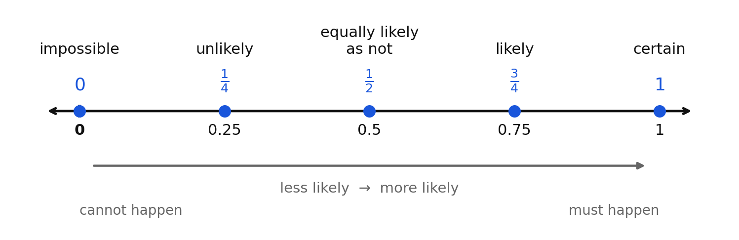
A probability of $\tfrac12$ means the event is equally likely as not — it has exactly as many favorable outcomes as unfavorable ones. Anything below $\tfrac12$ is unlikely; anything above is likely. If you ever compute a probability greater than 1 or less than 0, you have made an arithmetic error, not discovered a strange event.

The complement

The complement of an event is everything in the sample space that is not in the event. Since every outcome is either in the event or in its complement, the two probabilities must add to 1:

$$P(\text{not } E) = 1 - P(E)$$

For a fair die, $P(\text{even}) = \tfrac12$, so $P(\text{not even}) = 1 - \tfrac12 = \tfrac12$. For $P(3) = \tfrac16$, the complement is $P(\text{not }3) = 1 - \tfrac16 = \tfrac56$. The complement is often the faster route: counting the five faces that are not a 3 is more work than subtracting once.

Spinners: size is everything

A spinner is a circle divided into sectors with a pointer that is equally likely to stop anywhere around the circle. That means the probability of landing on a sector is the fraction of the circle's angle that the sector covers — not the fraction of the labels.

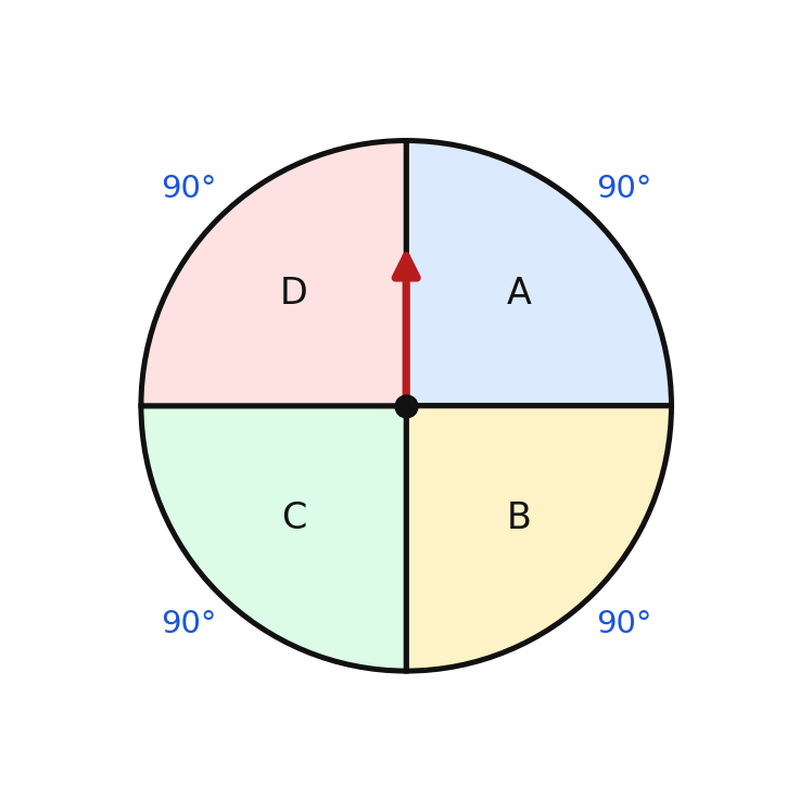
This spinner has four sectors, each spanning exactly $90°$, and $\tfrac{90}{360} = \tfrac14$. So $P(A) = P(B) = P(C) = P(D) = \tfrac14$. Here — and only here, because the sectors are equal — counting labels gives the right answer.

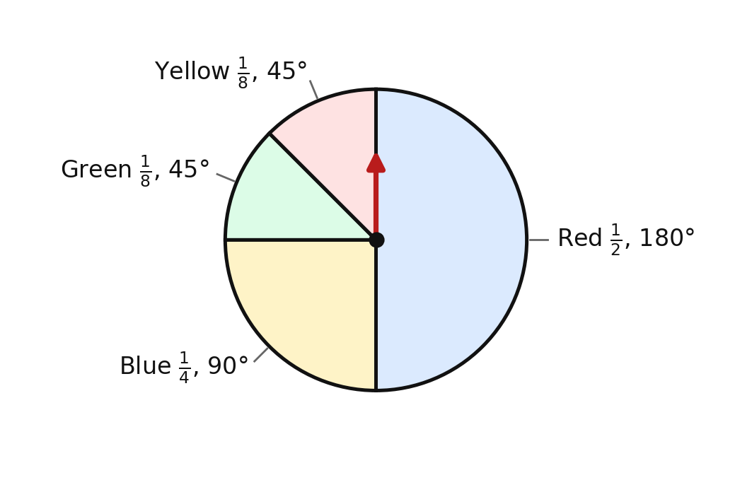
This second spinner also has four sectors, but they are not the same size, so the four outcomes are not equally likely and you cannot write $\tfrac14$ for any of them. Read the angles instead:

$$P(\text{red}) = \frac{180}{360} = \frac12 \qquad P(\text{blue}) = \frac{90}{360} = \frac14 \qquad P(\text{green}) = P(\text{yellow}) = \frac{45}{360} = \frac18$$

Check: $\tfrac12 + \tfrac14 + \tfrac18 + \tfrac18 = \tfrac48 + \tfrac28 + \tfrac18 + \tfrac18 = \tfrac88 = 1$. The probabilities of all the outcomes in a sample space always total exactly 1, and that sum is a free error check on every problem in this chapter.

Read the picture, not the count. The most common mistake with spinners is writing $\tfrac14$ because there are four colors. Four colors only means four equal chances when the four sectors are the same size.

Listing a sample space for two actions

When an experiment has two stages, the sample space is every combination of a first-stage outcome with a second-stage outcome. A tree diagram keeps the list organized so you do not miss any.

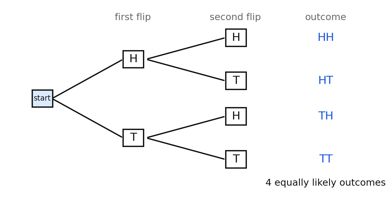
Flipping a coin twice has four equally likely outcomes: HH, HT, TH, TT. From that list you can read off any event you like.

$$P(\text{two heads}) = \frac14 \qquad P(\text{exactly one head}) = \frac{2}{4} = \frac12 \qquad P(\text{at least one head}) = \frac{3}{4}$$

HT and TH are genuinely different outcomes — heads then tails is not the same event as tails then heads — which is why "exactly one head" is twice as likely as "two heads."

Worked examples

Example 1 — A single outcome

A fair six-sided die is rolled once. Find $P(4)$ as a fraction, a decimal rounded to the nearest thousandth, and a percent rounded to the nearest tenth.

The sample space is $\{1,2,3,4,5,6\}$, six equally likely outcomes. One of them is a 4.

$$P(4) = \frac{1}{6} \approx 0.167 \approx 16.7\%$$

Answer: $\tfrac16$, about $0.167$, about $16.7\%$

Example 2 — An event with several outcomes

A fair six-sided die is rolled once. Find $P(\text{even})$.

The favorable outcomes are 2, 4, and 6 — three of the six.

$$P(\text{even}) = \frac{3}{6} = \frac12 = 0.5 = 50\%$$

Answer: $\tfrac12$

Example 3 — Using the complement

A bag holds 4 red marbles, 3 blue marbles, and 5 green marbles, all the same size and shape. One marble is drawn without looking. Find $P(\text{blue})$ and $P(\text{not blue})$.

There are $4 + 3 + 5 = 12$ marbles, so 12 equally likely outcomes.

$$P(\text{blue}) = \frac{3}{12} = \frac14$$ $$P(\text{not blue}) = 1 - \frac14 = \frac34$$

Check by counting directly: 4 red plus 5 green is 9 marbles that are not blue, and $\tfrac{9}{12} = \tfrac34$. The two routes agree.

Answer: $P(\text{blue}) = \tfrac14$; $P(\text{not blue}) = \tfrac34$

Example 4 — An unequal spinner

On the unequal spinner above, find $P(\text{green or yellow})$.

Green spans $45°$ and yellow spans $45°$, so together they span $90°$ of the $360°$ circle.

$$P(\text{green or yellow}) = \frac{45 + 45}{360} = \frac{90}{360} = \frac14$$

Equivalently, $\tfrac18 + \tfrac18 = \tfrac28 = \tfrac14$.

Answer: $\tfrac14$

Example 5 — The boundary cases

A fair six-sided die is rolled once. Find $P(\text{rolling a }10)$ and $P(\text{rolling a whole number from 1 to 6})$.

No face shows a 10, so there are zero favorable outcomes. Every face shows a whole number from 1 to 6, so all six are favorable.

$$P(10) = \frac{0}{6} = 0 \qquad P(\text{1 through 6}) = \frac{6}{6} = 1$$

Answer: $0$ (impossible) and $1$ (certain)

Guided practice

1. List the sample space for one roll of a fair six-sided die. How many outcomes does it contain?
2. For one roll of that die, find $P(3)$.
3. For one roll of that die, find $P(\text{odd})$. Write your answer in lowest terms.
4. On the spinner with four equal $90°$ sectors labeled A, B, C, and D, find $P(B)$.
5. A bag holds 4 red, 3 blue, and 5 green marbles. One marble is drawn without looking. Find $P(\text{red})$.
6. Using your answer to item 5 and the complement, find $P(\text{not red})$.

Independent practice

7. A fair six-sided die is rolled once. Find each probability in lowest terms. a) $P(5)$ b) $P(\text{greater than }4)$ c) $P(7)$ d) $P(\text{less than }7)$
8. A fair coin is flipped twice. List the four outcomes in the sample space, then find $P(\text{exactly one head})$ and $P(\text{two tails})$.
9. On the unequal spinner (red $180°$, blue $90°$, green $45°$, yellow $45°$), find $P(\text{red})$, $P(\text{blue})$, and $P(\text{green or yellow})$. Then show that all four sector probabilities add to 1.
10. From the bag of 4 red, 3 blue, and 5 green marbles, find $P(\text{green})$ and $P(\text{not green})$. Give each as a fraction in lowest terms, a decimal rounded to the nearest thousandth, and a percent rounded to the nearest tenth.
11. Eleven tiles are printed with the letters of the word PROBABILITY, one letter per tile, and one tile is drawn without looking. Find $P(\text{B})$ and $P(\text{vowel})$. Treat A, E, I, O, and U as the vowels.
12. A spinner has eight equal sectors numbered 1 through 8. Find $P(\text{a multiple of }3)$.
13. For one roll of a fair six-sided die, describe one event whose probability is $0$ and one event whose probability is $1$.
14. Place these four events for one roll of a fair die on the probability scale from 0 to 1, in order from least likely to most likely: rolling a 2; rolling a number greater than 0; rolling a number greater than 2; rolling a negative number.
15. Application. A raffle sells 25 tickets, and each ticket has an equal chance of being drawn as the single winner. Nadia buys 4 of them. Find the probability that Nadia wins, as a fraction, a decimal, and a percent.
16. Reasoning. Explain why the probabilities of all the outcomes in a sample space must add to exactly 1. Use the four-sector unequal spinner in your explanation.

Exit ticket 16.1

17. A fair six-sided die is rolled once. Find $P(2)$.
18. On the spinner with four equal sectors A, B, C, and D, find $P(A \text{ or } C)$.
19. From the bag of 4 red, 3 blue, and 5 green marbles, find $P(\text{blue})$ in lowest terms.
20. Explain the difference between an event with probability $0$ and an event with probability $1$, and give an example of each for a single die roll.

Lesson 16.2 — Experimental Probability

When reasoning is not enough

Theoretical probability requires you to know the sample space and to know the outcomes are equally likely. Plenty of real questions fail one of those conditions. What is the probability a thumbtack lands point up? That a particular basketball player makes a free throw? That a battery coming off an assembly line is defective? There is no tidy sample space of equally likely outcomes to count. For those questions you have to go and find out.

That is what SOL 7.PS.1 means by statistical investigation: you formulate a question, run the experiment many times, record what happens, and compute a probability from the record you built.

Trials, frequency, and the formula

One repetition of an experiment is a trial. The number of times a particular outcome occurs across all your trials is its frequency. A tally is the running record of marks you make as you go.

The experimental probability of an event — sometimes called the empirical probability — is

$$P_{\text{exp}}(\text{event}) = \frac{\text{number of trials in which the event occurred}}{\text{total number of trials}}$$

The structure is the same fraction as before, but the meaning is different in an important way. Theoretical probability comes from counting possibilities. Experimental probability comes from counting what actually happened. Nothing is predicted; something is measured.

A worked investigation: 60 rolls of a die

A class rolled one fair six-sided die 60 times and tallied the results.

First check the total, every time, before computing anything: $9 + 12 + 8 + 11 + 10 + 10 = 60$. If the frequencies do not add up to the number of trials, something was miscounted and no probability computed from the table can be trusted.

Now each experimental probability is that outcome's frequency over 60:

These six experimental probabilities also add to 1, because the six frequencies add to the 60 trials. That is the same free error check you used in Lesson 16.1.

For an event made of several outcomes, add the frequencies first and divide once:

$$P_{\text{exp}}(\text{even}) = \frac{12 + 11 + 10}{60} = \frac{33}{60} = \frac{11}{20} = 0.55$$

Reporting an experimental probability honestly

An experimental probability is meaningless without the number of trials attached to it. "The experimental probability of heads was $0.6$" could describe 3 heads in 5 flips or 600 heads in 1000, and those two results deserve very different amounts of trust. Always write the fraction with its real denominator — $\tfrac{3}{5}$ or $\tfrac{600}{1000}$ — before reducing it, so the number of trials stays visible.

Using experimental probability to predict

Once you have an experimental probability, you can use it to estimate how often the event would occur in a larger number of trials. Multiply the probability by the new number of trials.

If a shooter made 12 of 20 free throws, then $P_{\text{exp}}(\text{make}) = \tfrac{12}{20} = \tfrac35 = 0.6$, and in 100 attempts you would expect roughly $0.6 \times 100 = 60$ makes. "Roughly" is doing real work in that sentence: the prediction is an estimate built on an estimate, and the actual count will land somewhere near 60, not exactly on it.

Worked examples

Example 1 — From a coin record

A student flipped a fair coin 40 times and recorded 23 heads and 17 tails. Find the experimental probability of heads.

First check: $23 + 17 = 40$, so the record is complete.

$$P_{\text{exp}}(\text{heads}) = \frac{23}{40} = 0.575 = 57.5\%$$

Answer: $\tfrac{23}{40} = 0.575$

Example 2 — A single outcome from the 60-roll table

Using the class table above, find $P_{\text{exp}}(3)$.

The 3 came up 8 times in 60 trials.

$$P_{\text{exp}}(3) = \frac{8}{60} = \frac{2}{15} \approx 0.133$$

Answer: $\tfrac{2}{15}$, about $0.133$

Example 3 — An event with several outcomes

Using the same table, find $P_{\text{exp}}(\text{greater than }4)$.

Greater than 4 means a 5 or a 6, with frequencies 10 and 10.

$$P_{\text{exp}}(\text{greater than }4) = \frac{10 + 10}{60} = \frac{20}{60} = \frac13 \approx 0.333$$

Answer: $\tfrac13$

Example 4 — A spinner investigation

A student spun the four-equal-sector spinner 80 times and recorded A: 24, B: 17, C: 21, D: 18. Find $P_{\text{exp}}(A)$.

Check the total: $24 + 17 + 21 + 18 = 80$.

$$P_{\text{exp}}(A) = \frac{24}{80} = \frac{3}{10} = 0.3$$

Answer: $\tfrac{3}{10} = 0.3$

Example 5 — Predicting from experimental data

A factory inspected 400 batteries and found 12 defective. Find the experimental probability that a battery is defective, then estimate how many defective batteries to expect in a shipment of 5{,}000.

$$P_{\text{exp}}(\text{defective}) = \frac{12}{400} = \frac{3}{100} = 0.03 = 3\%$$ $$0.03 \times 5000 = 150$$

Answer: $0.03$, or $3\%$; expect about 150 defective batteries

Guided practice

21. Add the six frequencies in the 60-roll table and confirm the total is 60. Why must you do this before computing any probability?
22. Using the 60-roll table, find $P_{\text{exp}}(1)$ in lowest terms.
23. Using the 60-roll table, find $P_{\text{exp}}(6)$ in lowest terms.
24. Using the 60-roll table, find $P_{\text{exp}}(\text{greater than }4)$.
25. A coin was flipped 40 times, giving 23 heads and 17 tails. Find $P_{\text{exp}}(\text{tails})$.
26. A four-equal-sector spinner was spun 80 times, giving A: 24, B: 17, C: 21, D: 18. Find $P_{\text{exp}}(C)$.

Independent practice

27. Using the 60-roll table, find $P_{\text{exp}}(2)$, $P_{\text{exp}}(4)$, and $P_{\text{exp}}(5)$. Give each as a fraction in lowest terms and as a decimal rounded to the nearest hundredth.
28. Using the 60-roll table, find $P_{\text{exp}}(\text{odd})$. Then show that $P_{\text{exp}}(\text{odd}) + P_{\text{exp}}(\text{even}) = 1$ and explain why that had to happen.
29. Using the 80-spin spinner data (A: 24, B: 17, C: 21, D: 18), find $P_{\text{exp}}(B)$, $P_{\text{exp}}(D)$, and $P_{\text{exp}}(B \text{ or } D)$.
30. A different spinner was spun 50 times. The tally shows A: 14, B: 11, C: 13, and the count for D was smudged. Find the missing frequency for D, then find $P_{\text{exp}}(D)$.
31. A thumbtack was tossed 60 times and landed point up 33 times. Find $P_{\text{exp}}(\text{point up})$ and $P_{\text{exp}}(\text{point down})$ in lowest terms. Explain why theoretical probability cannot be used for this experiment.
32. A player made 12 of 20 free throws. Find $P_{\text{exp}}(\text{make})$, then estimate the number of makes in 100 attempts.
33. Application. An arcade game was played 250 times and awarded a prize 30 times. Find the experimental probability of winning a prize, as a fraction in lowest terms and as a percent.
34. Application. A quality inspector checked 400 phone cases and found 16 with scratches. Find $P_{\text{exp}}(\text{scratched})$ and estimate how many scratched cases to expect in a shipment of 2{,}500.
35. Reasoning. Explain why you cannot determine an experimental probability by thinking carefully about the situation, the way you can for theoretical probability.
36. Reasoning. Two students each flip the same fair coin 20 times. One records 9 heads and the other records 13 heads. Compute both experimental probabilities and explain how both records can be correct.

Exit ticket 16.2

37. A spinner was spun 30 times and landed on red 12 times. Find $P_{\text{exp}}(\text{red})$ in lowest terms.
38. Using the 60-roll table, find $P_{\text{exp}}(5)$.
39. A coin flipped 40 times gave 23 heads. Find $P_{\text{exp}}(\text{heads})$ as a decimal.
40. If the class rolled the same die 60 more times, would you expect the frequency table to come out identical? Explain what would change and what would stay the same.

Lesson 16.3 — What Happens as the Number of Trials Grows

One long investigation

Everything in this lesson comes from a single simulated investigation: one fair coin, flipped 1{,}000 times, with the running experimental probability of heads recorded along the way. The record below is real output from a computer simulation, not an idealized example, which is why it wobbles the way it does.

Each row is cumulative: the 200-flip row counts all 200 flips made so far, including the first 100.

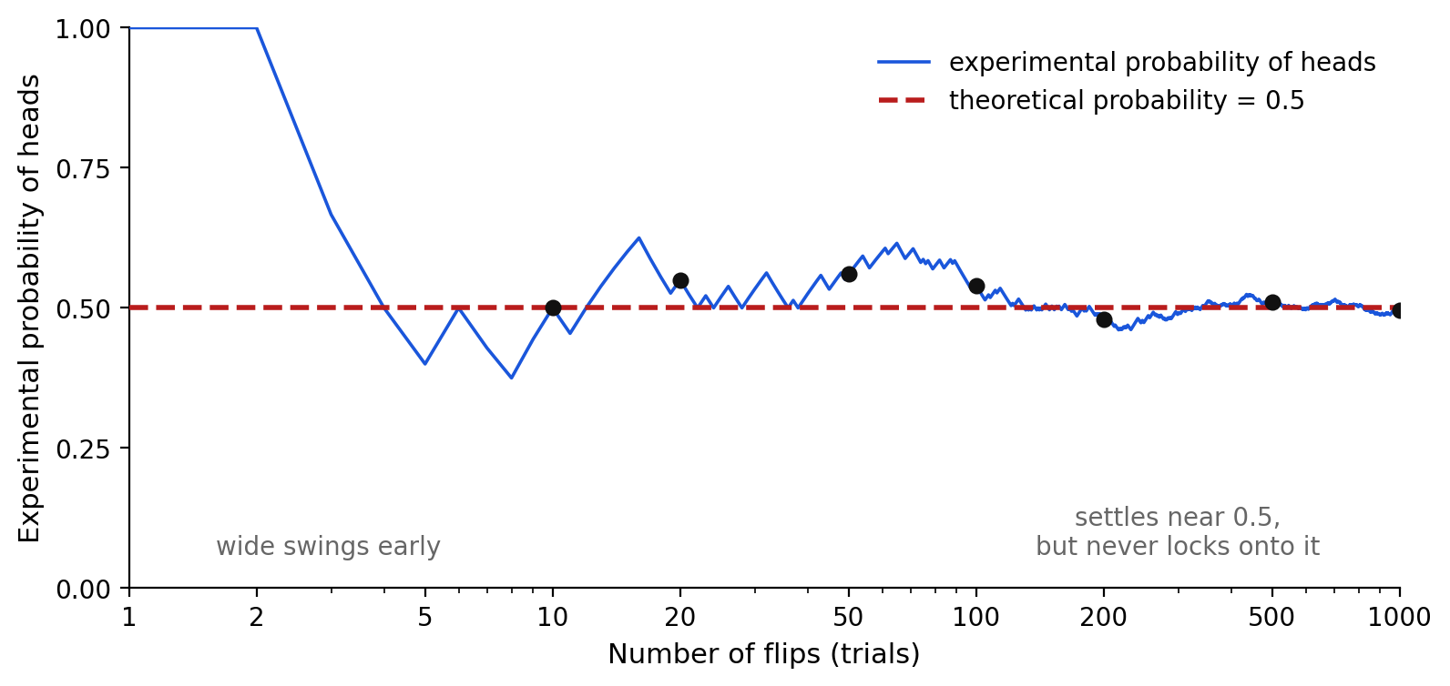
What the picture shows

Read the graph left to right. In the first few flips the curve is wild — it sits at $1.0$, then drops below $0.4$, then climbs again. With so few trials, one flip moves the fraction enormously: going from 3 heads in 4 flips to 3 heads in 5 flips drops the experimental probability from $0.75$ to $0.6$ in a single step.

Further right, the curve calms down and hugs the dashed line at $0.5$. By 500 flips one more head barely nudges the fraction at all. The honest summary is:

As the number of trials increases, the experimental probability tends to get closer to the theoretical probability.

Three words in that sentence are doing careful work, and every one of them matters.

What the picture does not show

"Tends to" is not "always." Look again at the table. After 10 flips the experimental probability was exactly $0.500$ — dead on. After 50 flips it was $0.560$, which is farther away. More trials did not improve the estimate at that step; it got worse before it got better. The tendency is real over the long run, but it is not a promise about any particular step.

"Closer" is not "equal." Even after 1{,}000 flips the experimental probability was $0.496$, not $0.5$. It never locks on. If you had stopped at 1{,}001 flips it would have moved again. There is no number of trials that makes the experimental probability equal the theoretical probability and stay there.

The gap in counts can grow while the gap in ratios shrinks. This is the part most people find surprising, and the table proves it. After 10 flips there were 5 heads and 5 was exactly half of 10, a count gap of 0. After 1{,}000 flips there were 496 heads where half of 1{,}000 is 500 — a count gap of 4. The number of "missing" heads went up, and yet the experimental probability got much closer to $0.5$, because 4 is a tiny share of 1{,}000 while any gap at all is a big share of 10.

Independence: the coin has no memory

Here is the single most important idea in the chapter, and the one most often gotten wrong.

Two events are independent when the outcome of one has no effect whatsoever on the outcome of the other. Coin flips are independent. Die rolls are independent. Spins of a spinner are independent.

Suppose you flip a fair coin and it comes up heads six times in a row. What is the probability the seventh flip is heads?

$$P(\text{heads}) = \frac12$$

Exactly the same as it was on the first flip. The coin is a piece of metal. It does not know what it did before, it is not keeping score, and it is not trying to even things out. There is no such thing as a flip being "due."

The false belief that a run of one outcome makes the other outcome more likely is common enough to have a name: the gambler's fallacy. It sounds reasonable — "it has to even out eventually" — and it is wrong. What actually happens is not that past results get cancelled out; it is that they get diluted. Those six heads are still there in the record forever. But after another 1{,}000 flips, six extra heads is a rounding error in the fraction, and the experimental probability drifts toward $0.5$ without anything ever pushing back the other way.

Say it precisely. Correct: "With more trials, the experimental probability tends to get closer to the theoretical probability." Incorrect: "With more trials, the experimental probability will equal the theoretical probability." Incorrect: "After five tails, heads is more likely."

Worked examples

Example 1 — Comparing two rows

Using the table above, find the experimental probability of heads after 50 flips and after 200 flips, and state which is closer to the theoretical value.

$$\frac{28}{50} = 0.56 \qquad \frac{96}{200} = 0.48$$ $$|0.56 - 0.5| = 0.06 \qquad |0.48 - 0.5| = 0.02$$

Answer: $0.56$ and $0.48$; the 200-flip result is closer, since $0.02 < 0.06$

Example 2 — When more trials did worse

The 10-flip row gave exactly $0.500$ and the 50-flip row gave $0.560$. What does this show about the claim "more trials always give a closer result"?

The distances are $0.000$ and $0.060$, so the estimate got worse when trials increased from 10 to 50.

Answer: It shows the claim is false. Landing exactly on $0.5$ after 10 flips was luck, not accuracy. More trials makes a close result more likely, but it does not guarantee improvement at every step.

Example 3 — The gambler's fallacy

A fair coin has landed heads six times in a row. Kenji says the next flip is more likely to be tails "to balance it out." Find the probability the next flip is heads and evaluate Kenji's reasoning.

Each flip is independent, so the six earlier flips have no effect on the seventh.

$$P(\text{heads on the next flip}) = \frac12$$

Answer: $\tfrac12$. Kenji is describing the gambler's fallacy. The coin has no memory; the run does not get cancelled, it gets diluted by later flips.

Example 4 — Count gap versus ratio gap

For the 100-flip row and the 1{,}000-flip row, find how far the number of heads is from exactly half the flips, and how far the experimental probability is from $0.5$.

At 100 flips: half of 100 is 50, and there were 54 heads, so the count gap is $|54 - 50| = 4$. The ratio gap is $|0.54 - 0.5| = 0.04$.

At 1{,}000 flips: half of 1{,}000 is 500, and there were 496 heads, so the count gap is $|496 - 500| = 4$. The ratio gap is $|0.496 - 0.5| = 0.004$.

Answer: The count gap stayed at 4 while the ratio gap shrank from $0.04$ to $0.004$, because the same gap is a much smaller share of a much larger number of trials.

Example 5 — Predicting the next stage

If the simulation continued to 4{,}000 flips, what would you expect the experimental probability of heads to be? Answer carefully.

Answer: It would most likely be closer to $0.5$ than the 1{,}000-flip value of $0.496$, and it would very likely be somewhere near $0.5$ — but it would almost certainly not be exactly $0.5$, and there is no guarantee it beats $0.496$. A larger sample makes a close result more likely without making it certain.

Guided practice

41. Using the table, find the experimental probability of heads after 100 flips as a fraction in lowest terms and as a decimal.
42. Find the distance from $0.5$ for the 20-flip row and for the 500-flip row. Which is closer?
43. Reading down the "distance from $0.5$" column, did the distance shrink at every single step? Name the step where it grew.
44. A fair coin lands heads six times in a row. Find the probability that the next flip is heads.
45. Find how far the number of heads is from exactly half the flips at 100 flips and at 1{,}000 flips.
46. Complete the sentence with the correct wording: "As the number of trials increases, the experimental probability ____________ the theoretical probability."

Independent practice

47. Using the table, write the 500-flip experimental probability as a fraction in lowest terms and as a decimal.
48. Order the 20-flip, 100-flip, and 1{,}000-flip rows from farthest from $0.5$ to closest to $0.5$. Show the three distances.
49. Owen says, "If you flip a fair coin 1{,}000 times, the experimental probability will be exactly $0.5$." Use the table to show he is wrong, and rewrite his statement so it is correct.
50. Priya has spun a spinner five times and gotten blue every time. She says blue is now less likely on the next spin. Explain what is wrong with her reasoning using the word independent.
51. A fair die is rolled 60 times and a 6 comes up 15 times. Find $P_{\text{exp}}(6)$ as a fraction in lowest terms and as a decimal. If the die is rolled 600 times, what would you expect the experimental probability to be, and how confident should you be?
52. A friend offers you two estimates of the same probability: one based on 30 trials and one based on 3{,}000 trials. Which would you trust more, and why? Is the one you chose guaranteed to be closer to the true value?
53. Application. A game company tests a new game twice. In a short test the game was played 20 times and won 8 times. In a long test it was played 200 times and won 46 times. Find both experimental probabilities and state which is the better estimate of the true win probability.
54. Application. A die is rolled 600 times and a 6 comes up 97 times. Find $P_{\text{exp}}(6)$ rounded to the nearest thousandth and compare it to the theoretical $\tfrac16$. Does this result suggest the die is unfair? Explain.
55. Reasoning. Explain in your own words what "the coin has no memory" means, and why it does not contradict the fact that the experimental probability drifts toward $0.5$.
56. Reasoning. Using the table, explain how the gap between the number of heads and half the flips can grow while the experimental probability gets closer to $0.5$.

Exit ticket 16.3

57. Using the table, which row has the experimental probability closest to $0.5$? Give the row and the distance.
58. A fair coin lands tails four times in a row. Find the probability the next flip is tails.
59. True or false: rolling a die enough times guarantees the experimental probability of a 6 will equal $\tfrac16$ exactly. Explain your answer.
60. In one sentence, describe what happens to the experimental probability as the number of trials increases. Be careful with your wording.

Lesson 16.4 — Comparing Theoretical and Experimental Probability

Two numbers for one event

You now have two ways to answer "how likely is this?" They come from completely different places.

For a fair die, $P(6) = \tfrac16$ no matter what — that number is a consequence of the die having six equal faces. But $P_{\text{exp}}(6)$ depends entirely on the 60 rolls you happened to make, and your neighbor's 60 rolls will give a different value.

Expected frequency

The cleanest way to compare the two is to convert the theoretical probability into a count you can hold up against your tally. The expected frequency of an event is

$$\text{expected frequency} = P(\text{event}) \times \text{number of trials}$$

For 60 rolls of a fair die, each face has expected frequency $\tfrac16 \times 60 = 10$. Now compare the class data from Lesson 16.2 against that expectation:

The differences always add to zero, because both rows add to the same 60 trials. That is another free error check.

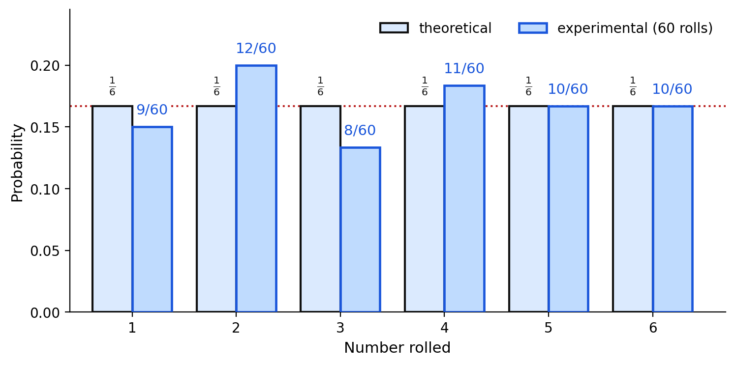
Every experimental bar sits near the dotted theoretical line without matching it, and no face is off by more than 2 rolls out of 60. That is exactly the picture a fair die produces.

Why they differ

There is no mystery here, and no error to hunt down. They differ because of variability — the natural, expected variation among random results. Sixty rolls of a perfectly fair die will almost never split 10-10-10-10-10-10, in the same way that sixty coin flips will almost never split exactly 30-30. Randomness is lumpy.

Two things follow.

A small difference is not evidence of anything. If your 60 rolls give nine 1s instead of ten, the die is not tilted. That is what fair dice do.

A large difference is evidence worth investigating. Suppose 60 rolls produced thirty-four 6s. Then $P_{\text{exp}}(6) = \tfrac{34}{60} = \tfrac{17}{30} \approx 0.567$, against an expected frequency of 10. A gap that size does not happen by chance with a fair die in any realistic sense, so the sensible conclusion is that the die is not fair — perhaps weighted. This is how experimental probability earns its keep: it is the only way to test whether a theoretical model actually describes the object in front of you.

They can also match exactly, by coincidence. In the 60-roll table, $P_{\text{exp}}(\text{greater than }4) = \tfrac{10+10}{60} = \tfrac13$, which is precisely the theoretical $\tfrac{2}{6} = \tfrac13$. An exact match is a pleasant accident, not a sign that the experiment was done especially well.

Simulation

A simulation is a model of a real experiment that uses some other random device to stand in for the original. It gives you experimental data without the original object.

To simulate rolls of a fair die you need six equally likely outcomes. A random number generator set to produce whole numbers from 1 to 6 works. So does a list of random digits, if you agree in advance to read digits 1 through 6 as rolls and simply skip 7, 8, 9, and 0 — skipping is essential, because the six digits you keep must remain equally likely.

To simulate the coin in Lesson 16.3 you need two equally likely outcomes: even digits could stand for heads and odd digits for tails, giving each a probability of $\tfrac12$. The 1{,}000-flip record in that lesson was produced exactly this way, by a computer.

Simulation is how people study experiments that would be too slow, too expensive, or too dangerous to run for real. What it produces is still experimental probability, with all the variability that comes with it — a simulation of 20 trials is just as unreliable as 20 real trials.

Worked examples

Example 1 — Comparing the two probabilities for one outcome

Using the 60-roll class data, compare the theoretical and experimental probabilities of rolling a 2.

$$P(2) = \frac16 \approx 0.167 \qquad P_{\text{exp}}(2) = \frac{12}{60} = \frac15 = 0.2$$

Answer: Theoretical $\tfrac16 \approx 0.167$; experimental $\tfrac15 = 0.2$. The experimental value is higher by about $0.033$, a small difference consistent with a fair die.

Example 2 — Expected frequency

How many 5s would you expect in 60 rolls of a fair die? Compare with the class data.

$$\text{expected frequency} = \frac16 \times 60 = 10$$

The class rolled ten 5s.

Answer: Expect 10; the class got 10, a difference of 0. This is a coincidence worth noticing but not a sign that the experiment was better run.

Example 3 — Comparing an event with several outcomes

Compare $P(\text{even})$ and $P_{\text{exp}}(\text{even})$ for the class data.

$$P(\text{even}) = \frac{3}{6} = \frac12 = 0.5$$ $$P_{\text{exp}}(\text{even}) = \frac{12 + 11 + 10}{60} = \frac{33}{60} = \frac{11}{20} = 0.55$$

Answer: $0.5$ versus $0.55$, a difference of $0.05$ — three more even rolls than the 30 expected.

Example 4 — Coins

A fair coin is flipped 40 times and comes up heads 23 times. Find the expected frequency of heads and the difference from the actual count, then compare the two probabilities.

$$\text{expected frequency} = \frac12 \times 40 = 20 \qquad 23 - 20 = 3$$ $$P(\text{heads}) = \frac12 = 0.5 \qquad P_{\text{exp}}(\text{heads}) = \frac{23}{40} = 0.575$$

Answer: Expect 20 heads; got 23, three more than expected. The probabilities are $0.5$ and $0.575$, differing by $0.075$ — an ordinary result for only 40 flips.

Example 5 — Deciding whether a model fits

Two students each spin a four-equal-sector spinner 80 times. Ana records A: 24, B: 17, C: 21, D: 18. Bea records A: 60, B: 6, C: 7, D: 7. Each sector has theoretical probability $\tfrac14$. What should each student conclude?

Expected frequency for each sector is $\tfrac14 \times 80 = 20$.

Ana's counts total $24 + 17 + 21 + 18 = 80$, and her differences from 20 are $+4$, $-3$, $+1$, $-2$. All are small.

Bea's counts total $60 + 6 + 7 + 7 = 80$, and her differences are $+40$, $-14$, $-13$, $-13$. Her $P_{\text{exp}}(A) = \tfrac{60}{80} = \tfrac34$, three times the theoretical $\tfrac14$.

Answer: Ana's data are consistent with four equal sectors. Bea's are not — a gap that large points to something wrong with the model or the equipment, such as a spinner whose sectors are not actually equal or a pointer that sticks.

Guided practice

61. For one roll of a fair die, state $P(3)$. Then find $P_{\text{exp}}(3)$ from the 60-roll class table and give the difference as a decimal rounded to the nearest thousandth.
62. Find the expected frequency of rolling a 5 in 60 rolls of a fair die.
63. The class rolled twelve 2s in 60 rolls. Find the difference between that frequency and the expected frequency.
64. Compare $P(\text{even})$ and $P_{\text{exp}}(\text{even})$ for the 60-roll class data.
65. A fair coin is flipped 40 times. Find the expected frequency of heads, then find the difference from the actual 23 heads.
66. A four-equal-sector spinner is spun 80 times. Find the expected frequency for sector A, then find the difference from Ana's actual 24.

Independent practice

67. Copy and complete this comparison table for the 60-roll class data. Give the experimental probability as a fraction and as a decimal rounded to the nearest thousandth, and the difference from the theoretical $\tfrac16 \approx 0.167$.

    Outcome	1	3	4
    Frequency out of 60
    $P_{\text{exp}}$ as a fraction
    $P_{\text{exp}}$ as a decimal
    Difference from $0.167$

68. For the 60-roll class data, compare $P(\text{greater than }4)$ with $P_{\text{exp}}(\text{greater than }4)$. Explain what an exact match does and does not tell you.

69. Using the 500-flip row from Lesson 16.3 (255 heads), find the expected frequency of heads and the difference from the actual count.

70. A bag holds 4 red, 3 blue, and 5 green marbles. A marble is drawn and replaced 120 times. Find the expected frequency of green.

71. Describe how you would use a random number generator to simulate 100 spins of the four-equal-sector spinner. Say exactly which numbers stand for which sectors.

72. A die is rolled 60 times and a 6 comes up 34 times. Find $P_{\text{exp}}(6)$ in lowest terms and as a decimal rounded to the nearest thousandth. Compare it to $\tfrac16$ and say whether the die is likely fair.

73. Devon says a well-run experiment should produce an experimental probability equal to the theoretical probability, and that any difference means someone counted wrong. Explain what Devon is missing.

74. Application. A game advertises that $\tfrac15$ of all plays win a prize. A club plays the game 300 times and wins 41 times. Find the expected frequency of wins, find $P_{\text{exp}}(\text{win})$ rounded to the nearest thousandth, and comment on whether the advertisement looks accurate.

75. Application. A cereal company says $\tfrac16$ of its boxes contain a prize. A store opens 90 boxes and finds 14 prizes. Find the expected frequency, find $P_{\text{exp}}(\text{prize})$ rounded to the nearest thousandth, and say whether this result is consistent with the company's claim.

76. Reasoning. Give two reasons an experimental probability can differ from the theoretical probability of the same event.

77. Reasoning. Explain how you would decide whether a difference between experimental and theoretical probability is ordinary variability or evidence that the theoretical model is wrong.

78. Reasoning. Can an event with theoretical probability greater than 0 have an experimental probability of exactly 0? Give an example with numbers and explain.

Exit ticket 16.4

79. State $P(1)$ for a fair die, then find $P_{\text{exp}}(1)$ from the 60-roll class table.
80. Find the expected frequency of heads in 200 flips of a fair coin, and compare it with the 96 heads recorded in the Lesson 16.3 table.
81. A four-equal-sector spinner is spun 40 times and lands on A ten times. Compare the theoretical and experimental probabilities of landing on A.
82. In two or three sentences, explain the difference between theoretical and experimental probability, and name one situation in which only the experimental probability can be found.

Chapter 16 Review

Vocabulary. probability experiment · outcome · sample space · event · favorable outcome · equally likely · theoretical probability · impossible event · certain event · complement · tree diagram · trial · frequency · tally · statistical investigation · experimental probability · independent · gambler's fallacy · expected frequency · variability · simulation

Part A — Theoretical probability (7.PS.1a)

83. A fair six-sided die is rolled once. Find $P(3)$, $P(\text{odd})$, and $P(\text{less than }3)$, each in lowest terms.
84. A bag holds 4 red, 3 blue, and 5 green marbles. Find $P(\text{red})$, $P(\text{blue})$, and $P(\text{not green})$.
85. On the spinner with red $180°$, blue $90°$, green $45°$, and yellow $45°$, find $P(\text{red})$ and $P(\text{green or yellow})$.
86. A fair coin is flipped twice. List the sample space, then find $P(\text{two heads})$ and $P(\text{at least one head})$.
87. For one roll of a fair die, name one event with probability $0$ and one event with probability $1$.
88. A spinner has eight equal sectors numbered 1 through 8. Find $P(\text{greater than }5)$.
89. An event $E$ has $P(E) = \tfrac27$. Find $P(\text{not } E)$.

Part B — Experimental probability (7.PS.1b)

A fair six-sided die was rolled 100 times in a statistical investigation, with these results. Use this table for items 90 through 94.

90. Find $P_{\text{exp}}(2)$ as a fraction and as a decimal.
91. Find $P_{\text{exp}}(6)$ in lowest terms.
92. Find $P_{\text{exp}}(\text{even})$ in lowest terms.
93. Find $P_{\text{exp}}(\text{odd})$ in lowest terms, and show that it and $P_{\text{exp}}(\text{even})$ add to 1.
94. Find $P_{\text{exp}}(\text{less than }3)$.
95. A coin was flipped 80 times and came up heads 37 times. Find $P_{\text{exp}}(\text{heads})$ and $P_{\text{exp}}(\text{tails})$ as decimals.

Part C — Changes as the number of trials increases (7.PS.1c)

96. Using the 1{,}000-flip table from Lesson 16.3, find the distance from $0.5$ at 20 flips and at 1{,}000 flips.
97. Which is the better estimate of the true probability of heads: the 10-flip result or the 1{,}000-flip result? Explain, and account for the fact that the 10-flip result was exactly $0.5$.
98. A fair coin lands heads seven times in a row. Find the probability the next flip is heads.
99. True or false: after enough flips, the experimental probability of heads becomes exactly $0.5$. Explain.
100. Write one careful sentence describing what happens to the experimental probability as the number of trials increases.

Part D — Comparing experimental and theoretical probability (7.PS.1d)

101. Using the 100-roll table in Part B, compare $P(3)$ with $P_{\text{exp}}(3)$. Give the difference as a decimal rounded to the nearest thousandth.
102. Find the expected frequency of each outcome in 100 rolls of a fair die, rounded to the nearest tenth. Then name the outcome in the Part B table whose actual frequency is farthest from it.
103. Find the expected frequency of heads in 80 flips of a fair coin, and compare it with the 37 heads in item 95.
104. A die is rolled 120 times and a 6 comes up 42 times. Find the expected frequency of 6s and $P_{\text{exp}}(6)$ in lowest terms. Is this die likely fair? Explain.
105. Describe how to simulate 100 rolls of a fair die using random digits, including what to do with digits 7, 8, 9, and 0.

Part E — Mixed application and reasoning

106. Application. A raffle sells 250 tickets and draws one winner, with every ticket equally likely. Trey buys 10 tickets. Find $P(\text{Trey wins})$ and $P(\text{Trey does not win})$, each in lowest terms and as a percent.
107. Application. The unequal spinner (red $\tfrac12$, blue $\tfrac14$, green $\tfrac18$, yellow $\tfrac18$) was spun 400 times, giving red 191, blue 108, green 45, yellow 56. Verify the frequencies total 400. Find the expected frequency of each color and $P_{\text{exp}}(\text{red})$ as a decimal. Are these results consistent with the stated sector sizes?
108. Reasoning. Explain why no probability can equal $1.4$ or $-0.2$.
109. Reasoning. After the spinner in item 107 landed on red four times in a row, a player says red is now less likely on the next spin. Explain why this is wrong, using the word independent, and state the correct probability for the next spin.
110. Reasoning. Explain the difference between theoretical and experimental probability, and describe one situation in which only experimental probability can be determined.

Standards coverage check — Chapter 16

How the statistical-investigation requirement is met. The standard frames probability through statistical investigation, so students do not only compute ratios. Lesson 16.2 works from complete trial records — 60 die rolls, 40 coin flips, 80 spinner spins — that students also generate themselves in the workbook. Lesson 16.3 works from a 1{,}000-flip simulated investigation, reported at seven cumulative checkpoints. Lesson 16.4 compares those records against theoretical expectations and introduces simulation as a way to acquire trial data.

Conceptual guardrails. Bullet c is stated throughout as a tendency, never a guarantee: the experimental probability tends to get closer to the theoretical probability as trials increase, individual short runs can differ a great deal, and the two never lock together. Independence is stated explicitly in Lesson 16.3, and the gambler's fallacy is named and refuted in the narrative (items 44, 50, 58, 98, and 109).

Scope note. Compound probability with the multiplication rule, conditional probability, and permutations and combinations are not part of 7.PS.1 and are deliberately absent. The two-coin tree diagram in Lesson 16.1 is used only to list a sample space, so every probability computed from it still comes from counting equally likely outcomes.

Answer keys for every set in this chapter are in Appendix A.