Chapter 19 — The Data Cycle: Scatterplots and Curve of Best Fit
Standard: A.ST.1 (a–i)
A.ST.1 — verbatim. The student will apply the data cycle (formulate questions; collect or acquire data; organize and represent data; and analyze data and communicate results) with a focus on representing bivariate data in scatterplots and determining the curve of best fit using linear and quadratic functions. Students will demonstrate the following Knowledge and Skills: a) Formulate investigative questions that require the collection or acquisition of bivariate data. b) Determine what variables could be used to explain a given contextual problem or situation or answer investigative questions. c) Determine an appropriate method to collect a representative sample, which could include a simple random sample, to answer an investigative question. d) Given a table of ordered pairs or a scatterplot representing no more than 30 data points, use available technology to determine whether a linear or quadratic function would represent the relationship, and if so, determine the equation of the curve of best fit. e) Use linear and quadratic regression methods available through technology to write a linear or quadratic function that represents the data where appropriate and describe the strengths and weaknesses of the model. f) Use a linear model to predict outcomes and evaluate the strength and validity of these predictions, including through the use of technology. g) Investigate and explain the meaning of the rate of change (slope) and -intercept (constant term) of a linear model in context. h) Analyze relationships between two quantitative variables revealed in a scatterplot. i) Make conclusions based on the analysis of a set of bivariate data and communicate the results.
By the end of this chapter you will be able to:
- Apply the data cycle to bivariate questions: formulate, collect or acquire, organize and represent, analyze and communicate (A.ST.1a–c, i)
- Write an investigative question that needs two paired measurements (A.ST.1a)
- Choose independent and dependent variables that fit a situation (A.ST.1b)
- Name an appropriate sampling method, including a simple random sample, and say why it matters (A.ST.1c)
- Read a scatterplot of no more than 30 points and describe the association (A.ST.1h)
- Use technology to decide whether a linear or quadratic curve of best fit is appropriate, and obtain its equation (A.ST.1d, e)
- Use a linear model to predict, and judge whether the prediction is honest (A.ST.1f)
- Interpret the slope and -intercept of a linear model in context, with units (A.ST.1g)
- State conclusions carefully — including that association is not causation (A.ST.1i)
Lessons: 19.1 The Data Cycle and Bivariate Questions · 19.2 Choosing Variables and Sampling · 19.3 Analyzing Relationships in a Scatterplot · 19.4 Technology: Linear or Quadratic Fit · 19.5 Regression Models and Predictions · 19.6 Interpreting Parameters and Communicating Conclusions
Why this chapter matters. Chapters 5–7 taught you to read a linear function: slope, intercepts, domain. Chapters 15–16 taught you to solve and graph quadratics. This chapter asks a different question of the same families: given real paired data, which curve — if either — should technology fit, and what does that model honestly say? Grade 8 sketched a line of best fit by eye. Algebra 1 requires the graphing calculator (or equivalent technology) to produce the equation. You will never be asked to invent regression coefficients by hand.
Scope note. Every data set in this chapter is bivariate and has no more than 30 ordered pairs, as A.ST.1d requires. Curves of best fit are linear or quadratic only, obtained with technology. Sketching a line by eye is Grade 8 work and is not credited here as a regression. Exponential models, correlation coefficients as graded answers, and formal residual analysis are outside this standard.
Conventions this chapter fixes.
- Regression coefficients are reported rounded to the nearest hundredth, with the words technology or from technology in the answer. A different calculator model may differ in the last digit; that is a rounding difference, not an error.
- A predicted value from a model is written (read "y-hat") when it helps to separate a prediction from an observed .
- Interpolation means predicting for an inside the data's horizontal span. Extrapolation means predicting outside that span — less trustworthy, and you must say so.
- Association is not causation. Every conclusion that reports a relationship also refuses the leap from "tends to" to "causes," unless an experiment assigned the treatments.
- Item numbering runs straight through the chapter, from 1 in Lesson 19.1 to 124 at the end of the review. It does not restart at each lesson.
Lesson 19.1 — The Data Cycle and Bivariate Questions
The same four stages, aimed at two variables
The data cycle has not changed since Grade 7:
- Formulate questions.
- Collect or acquire data.
- Organize and represent data.
- Analyze data and communicate results.
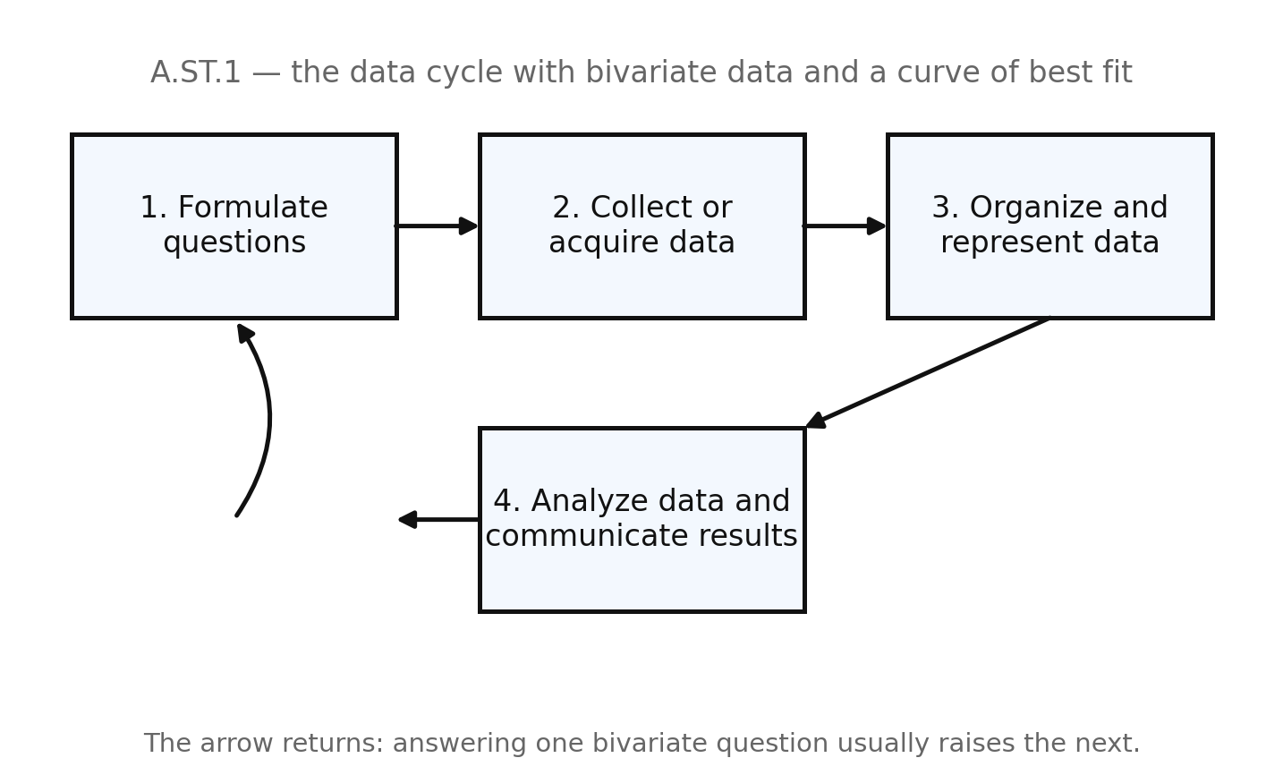
What is new in Algebra 1 is the focus: every question in this chapter needs bivariate data — two quantitative measurements kept paired as ordered pairs — and the analysis stage ends with a curve of best fit obtained from technology when a linear or quadratic model is appropriate.
What makes a question bivariate
A question is bivariate when answering it requires two numbers for each item, kept together.
| Question | Why it is (or is not) bivariate |
|---|---|
| "How many hours do Algebra 1 students study in a week?" | Univariate — one number per student |
| "For Algebra 1 students in our school, is there a relationship between hours studied in a week and exam score?" | Bivariate — two numbers per student, paired |
| "What is the average resale value of used cars on the lot?" | Univariate |
| "For used cars on this lot, how does resale value relate to the age of the car?" | Bivariate |
A.ST.1a asks you to formulate investigative questions of the second kind: questions that require collecting or acquiring bivariate data.
Anatomy of a good investigative question
A usable question names four things:
- The population (or the group you can actually reach)
- Both quantitative variables
- That you are asking about a relationship (or about how one tends to change with the other)
- Enough context that another student could collect the same kind of data
Weak: "Does studying help?" Strong: "For Algebra 1 students at Lincoln High, is there a relationship between the number of hours a student studies in a week and that student's score on the unit exam?"
Worked examples
Example 1 — Naming a stage
A class writes: "For ninth graders in our school, is there a relationship between minutes of sleep last night and reaction time on a phone app?" Which stage is this?
They are deciding what they want to know and putting it in words that demand two paired measurements.
Answer: Formulate questions (A.ST.1a).
Example 2 — Bivariate or not
"What is the typical commute time for students at our school?" Is this bivariate?
Only one measurement per student is named.
Answer: No — it is univariate. A bivariate version would pair commute time with a second quantity, such as distance from school.
Example 3 — Repairing a question
Repair: "Are phones bad?"
The original names neither population nor variables.
Answer: One acceptable repair: "For students in our Algebra 1 class, is there a relationship between hours of phone use the night before a quiz and the quiz score?"
Example 4 — Naming a stage
The class enters 18 ordered pairs into a graphing calculator and displays a scatterplot. Which stage?
Making the pairs visible is the third stage.
Answer: Organize and represent data.
Example 5 — Why pairing matters
A student says, "I have a list of 20 study times and a separate list of 20 exam scores, so I have bivariate data." What is wrong?
Two separate lists are two univariate sets unless each study time stays matched to the score of the same student.
Answer: Without the pairing you cannot form ordered pairs, plot points, or fit a curve. Bivariate data keeps the two measurements locked together.
Example 6 — Closing the cycle
After fitting a line, a student asks whether where students studied matters too. Which stage is starting again?
A new investigative question has been born.
Answer: Formulate questions — the cycle returns to the beginning.
Guided practice
- Name the four stages of the data cycle in order.
- What makes a data set bivariate?
- Which stage is shown when a class writes a question that requires two paired measurements?
- Is "How tall are the players on the basketball team?" a bivariate investigative question? Explain.
- Rewrite "Does advertising work?" as a bivariate investigative question that names a population and two quantitative variables.
- A student says the data cycle ends once technology produces a regression equation. Correct the statement.
Independent practice
- Name the stage for each action. a) Measuring both the length and the mass of each of 16 metal rods b) Writing "For seedlings in our greenhouse, is there a relationship between days since planting and height in centimeters?" c) Entering 16 ordered pairs and displaying a scatterplot on a graphing calculator d) Reporting to the class that taller seedlings tended to be the ones planted earlier, and stating the linear model from technology
- These stages are scrambled. Put them in order: organize and represent data; analyze data and communicate results; formulate questions; collect or acquire data.
- For each, state whether the question is univariate or bivariate. If univariate, rewrite it as bivariate. a) "How many minutes do students exercise each day?" b) "For adults in a clinic study, how does resting heart rate relate to age?" c) "What is the mass of each backpack in the classroom?" d) "For backpacks in the classroom, how does mass relate to the number of books inside?"
- Application. Write one bivariate investigative question your class could actually answer in a week, naming the population and both variables.
- Reasoning. Explain why "Is there a relationship between happiness and success?" fails as an A.ST.1a question even though it mentions two ideas.
- Error analysis. A student lists 25 heights in one column and 25 arm spans in another, shuffled independently, then asks the calculator for a linear regression. Identify the error.
Exit ticket 19.1
- Name the four stages of the data cycle.
- Write a bivariate investigative question about practice time and free throws made.
- Which stage are you in when you choose a simple random sample of 20 students and record two measurements for each?
- Explain in one sentence why bivariate data requires that the two measurements stay paired.
Lesson 19.2 — Choosing Variables and Sampling
Which variables could explain the situation
A.ST.1b asks you to determine what variables could be used to explain a situation or answer an investigative question. That is a design choice, made before you collect.
- The independent variable () is the input you think of as explanatory — the one set first, measured as a predictor, or suspected of doing the explaining.
- The dependent variable () is the response.
For "hours studied" and "exam score," hours studied is and score is . Swapping them does not break the scatterplot, but it changes the story the regression will tell, and readers expect the explanatory variable on the horizontal axis.
Often more than one pair of variables could address the same rough idea. "Does studying pay off?" might use hours studied vs. exam score, or pages of notes vs. exam score, or days attended vs. exam score. A.ST.1b wants you to name variables that are quantitative, measurable, and matched to the question.
Collecting a representative sample
A.ST.1c asks for an appropriate method to collect a representative sample, and it names simple random sample as one such method.
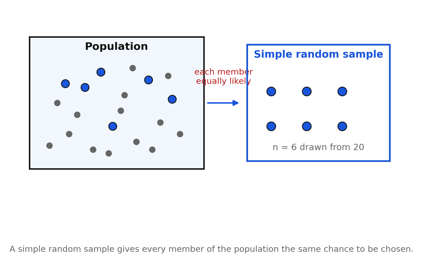
In a simple random sample (SRS), every member of the population has the same chance of being chosen, and every sample of the planned size is equally likely. Technology can draw an SRS (random integer generators, sampling features); so can well-mixed slips in a hat. Convenience samples — "whoever is in the cafeteria right now" — are easy and often biased.
Other appropriate methods exist (stratified samples, systematic samples, using an existing trustworthy data source). This chapter expects you to name a method, say why it fits, and recognize when a method is likely to misrepresent the population.
Worked examples
Example 1 — Choosing variables
Situation: a coach wonders whether more practice relates to fewer turnovers in games. Name quantitative variables for and .
Practice is the explanatory idea; turnovers are the response.
Answer: = hours of practice in a week (or minutes); = number of turnovers in the next game. (Other measurable pairs are acceptable if both are quantitative and matched.)
Example 2 — A bad variable choice
A student proposes = "motivation" on a vague 1–3 feeling scale invented during the quiz, and = exam score. What is the problem for A.ST.1b?
"Motivation" here is not a clearly measurable quantitative variable tied to a reproducible procedure.
Answer: Choose a measurable proxy (for example, hours of study logged) so another class could collect the same kind of data.
Example 3 — SRS
A school has 400 Algebra 1 students. You need 25 for a bivariate study. Describe an SRS.
Answer: Number the 400 students to . Use a calculator's random-integer feature (or an equivalent tool) to select distinct numbers, then record both measurements for those students. Every student had the same chance to be chosen.
Example 4 — Not representative
A class surveys only the students who stay after school for tutoring, then claims the results describe all Algebra 1 students. What went wrong?
Answer: The sample is a convenience sample of students already seeking extra help — likely not representative of the whole Algebra 1 population.
Example 5 — Existing source
A class uses a published NOAA table of daily high temperature and energy demand for a city, with paired days. Is that "collect or acquire"?
Answer: Acquire — the data already exist. The method can still be appropriate if the source is trustworthy and the pairs stay matched. The set must still have no more than points for the regression work in this standard.
Example 6 — Method choice
You want opinions from each grade 9–12 in equal share. Why might a stratified sample fit better than a pure SRS of the whole school?
Answer: An SRS of the whole school might by chance under-represent one grade. Stratifying by grade, then drawing randomly within each grade, keeps each grade represented.
Guided practice
- In a study of car age and resale value, which variable belongs on the horizontal axis, and what is it called?
- Name two different pairs of quantitative variables that could investigate whether "more sleep helps school performance."
- What is a simple random sample?
- A teacher picks the first students who walk into class. Is this an SRS? Explain.
- A club has members and wants an SRS of . Describe how to use technology to draw it.
- Why does A.ST.1 care whether a sample is representative?
Independent practice
- For each situation, name an appropriate independent variable and dependent variable. a) Fertilizer amount and tomato yield for greenhouse plants b) Outside temperature and cups of hot chocolate sold at the school store c) Weeks of advertising and weekly sales for a small shop
- A student wants to study phone use and sleep. Critique this plan: survey only the student's teammates on the soccer team, then generalize to all teens in the state.
- Application. Your class will study days since planting and seedling height for plants in the school greenhouse. Describe an appropriate sampling method if there are seedlings and you will measure .
- Application. Explain one strength and one weakness of using an existing public data set instead of collecting new measurements yourself.
- Reasoning. "Any sample of size is automatically representative." Explain why that is false.
- Error analysis. A student says the independent variable is whichever column the calculator plots first, so it does not matter which quantity you call . Identify what is wrong for interpreting the model later.
Exit ticket 19.2
- For hours charged and battery percent, name and .
- Define a simple random sample in one sentence.
- Give one reason a cafeteria convenience sample may fail to represent a school's Algebra 1 students.
- Name one appropriate method, other than an SRS, for obtaining bivariate data to answer an investigative question.
Lesson 19.3 — Analyzing Relationships in a Scatterplot
What a scatterplot shows
A scatterplot displays bivariate data: each item is one point . A.ST.1h asks you to analyze relationships between two quantitative variables revealed in that picture — before, and sometimes without, fitting a curve.
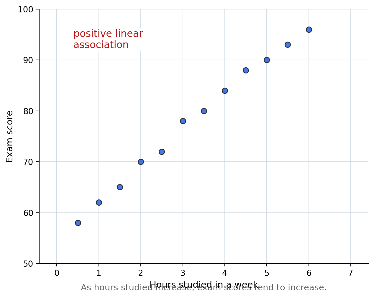
The study-time cloud climbs from lower left to upper right: a positive linear association. As increases, tends to increase, and the points lie roughly along a line.
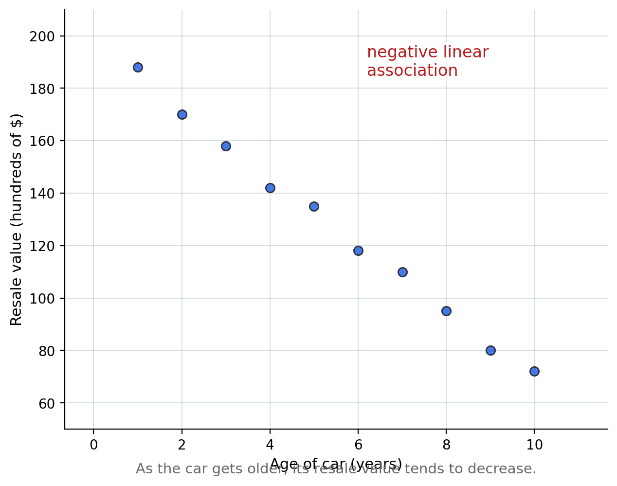
The car-age cloud falls from upper left to lower right: a negative linear association.
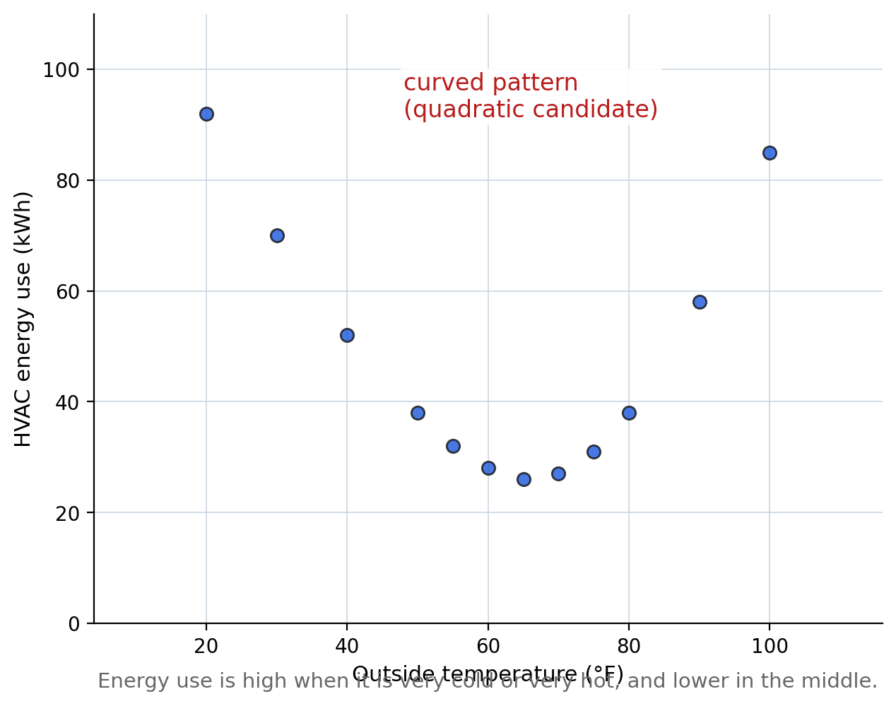
Energy use is high when it is very cold or very hot and lower in the middle: a curved pattern — a quadratic candidate. Linear language is not enough here.
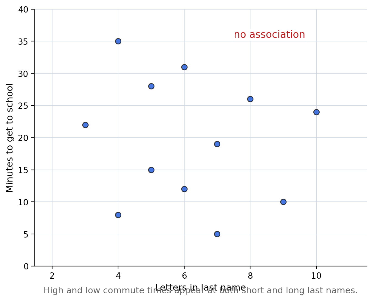
High and low commute times appear at both short and long names: no association. That is a real, reportable result.
How to justify what you see
A justification has three parts:
- Name the pattern (positive linear, negative linear, curved / quadratic candidate, or no association).
- Point at evidence in the plot (direction, clusters, specific points).
- Say what it means in context, with the actual quantities and units.
Association is not causation
A clear association does not prove that causes . A lurking variable may drive both, or the arrow of cause may run the other way, or the pattern may be coincidence in this sample. Report what the scatterplot supports: "tended to," not "causes," unless the study assigned treatments experimentally.
Worked examples
Example 1 — Naming the association
The points in the study figure climb steadily. Name the association.
Answer: Positive linear association.
Example 2 — Negative
In the car figure, what happens to resale value as age increases?
Answer: Resale value tends to decrease — negative linear association.
Example 3 — Curved
Why is "positive linear" wrong for the HVAC figure?
Answer: The cloud is U-shaped: falls then rises. A single linear direction does not describe the whole pattern.
Example 4 — No association
Justify "no association" for the name-length figure using two -values as evidence.
Answer: At the times are and minutes; at they are and . High and low values appear at both smaller and larger , so last-name length does not tend to push commute time up or down.
Example 5 — Context sentence
Write one context sentence for the study figure.
Answer: Algebra 1 students in this sample who studied more hours in a week tended to score higher on the exam.
Example 6 — Causation trap
A scatterplot of ice cream sales and sunburns shows a positive linear association. May you conclude that ice cream causes sunburns?
Answer: No. A lurking variable such as hot, sunny weather can push both up. The plot supports association, not causation.
Guided practice
Items 33–38 use the four figures in this lesson.
- Describe the association in the study-time scatterplot.
- Describe the association in the car-age scatterplot.
- Describe the pattern in the HVAC energy scatterplot, and say why a linear description is incomplete.
- Describe the association in the last-name scatterplot.
- Cite two points from the study figure that support a positive trend.
- Write one sentence that reports the car-age result without claiming causation.
Independent practice
Use this plant data (days since planting, height in cm) for items 39–42:
| Days () | 2 | 4 | 6 | 8 | 10 | 12 | 14 | 16 | 18 | 20 |
|---|---|---|---|---|---|---|---|---|---|---|
| Height () | 5 | 8 | 12 | 15 | 19 | 22 | 26 | 29 | 33 | 36 |
- How many ordered pairs are in the table? Does the set satisfy the chapter's 30-point limit?
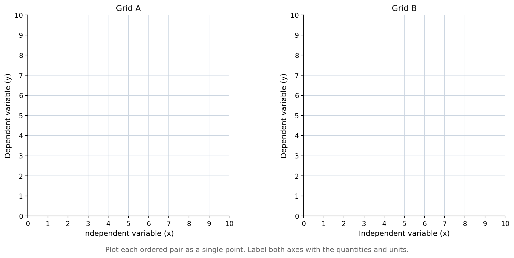
- On a blank grid, plot the plant data (or use Grid A in the blank-grids figure). Label both axes.
- Describe the association.
- Write a justification with evidence and a context sentence.
- Application. A classmate claims any U-shaped cloud is "no association" because it is not a straight line. Correct the claim.
- Reasoning. Explain why two students can both practice hours and appear as two separate points on a scatterplot, stacked vertically.
- Error analysis. A student says a scatterplot must pass the vertical-line test because "graphs of functions can't have two -values for one ." Identify the confusion.
Exit ticket 19.3
- Name the four pattern descriptions this lesson uses.
- The car-age cloud falls from left to right. Name the association and give a context sentence.
- Give one reason a curved pattern might suggest trying a quadratic model with technology.
- State the sentence "association is not causation" in your own words with one example.
Lesson 19.4 — Technology: Linear or Quadratic Fit
What A.ST.1d actually requires
Given a table or scatterplot of no more than 30 points, you must use available technology to decide whether a linear or quadratic function would represent the relationship, and if so, to obtain the equation of the curve of best fit.
That means:
- Enter the paired data into a graphing calculator, Desmos (Virginia), spreadsheet, or equivalent.
- Display the scatterplot.
- Look at the cloud — and, when your tool offers both, compare a linear fit with a quadratic fit.
- Choose the model that follows the pattern (or conclude that neither linear nor quadratic is appropriate).
- Record the equation from technology, coefficients rounded to the nearest hundredth.
You do not compute least-squares coefficients by hand in this course. Showing a sketched line without technology does not satisfy A.ST.1d.
When the linear fit is the wrong tool
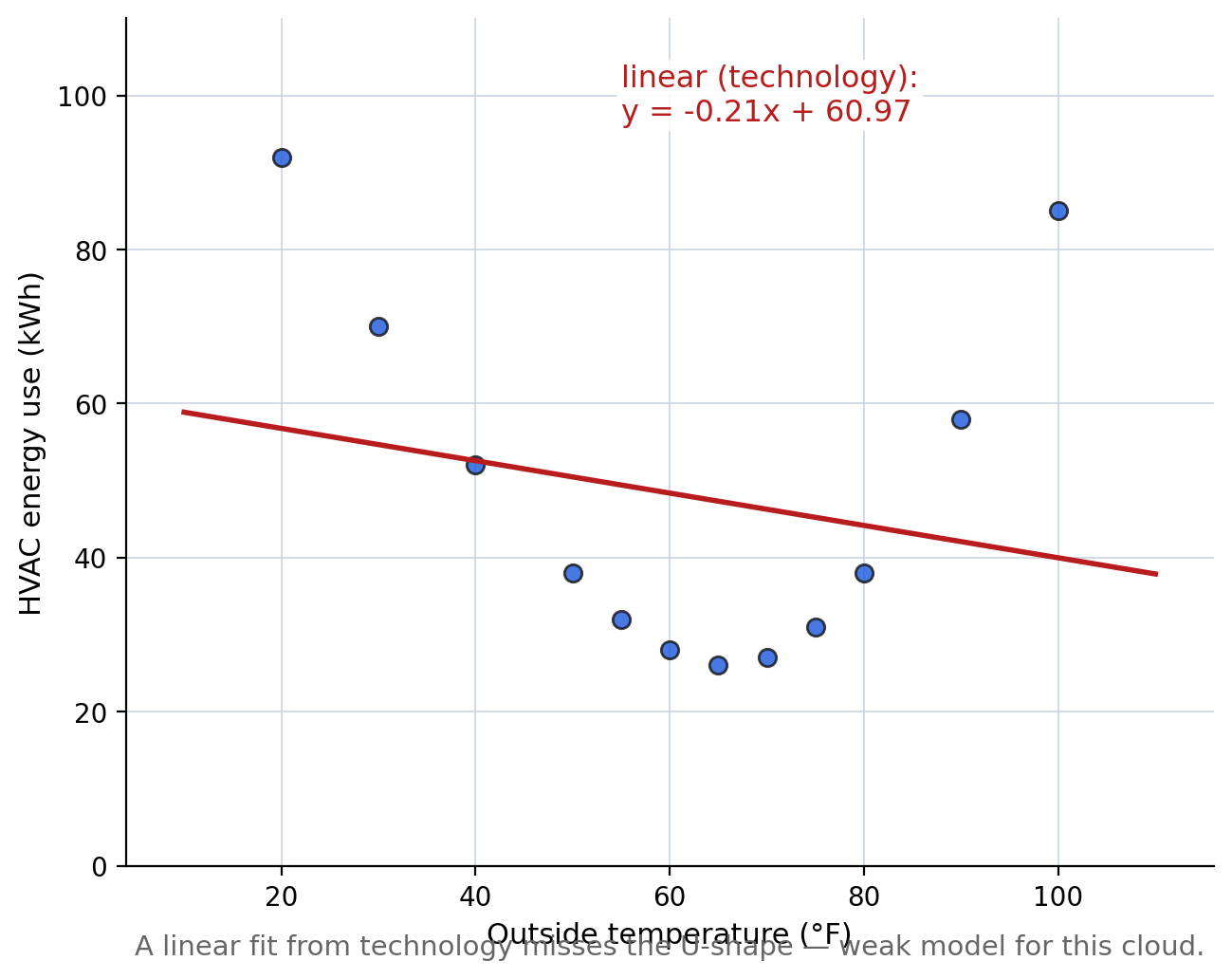
Technology will happily return a linear equation for the HVAC data: . The line is almost flat and cuts through the middle while the points dive and climb around it. The tool did the arithmetic; you still have to reject the model because it does not represent the relationship.
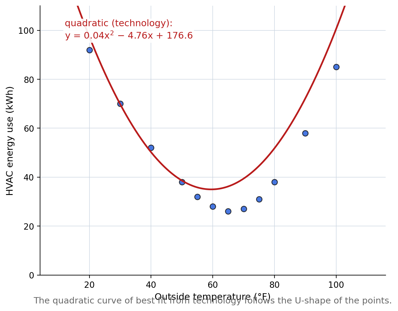
The quadratic from technology, , follows the U-shape. That is the curve of best fit A.ST.1d is asking for on this set.
A checklist for choosing
| What you see | Technology move | Decision |
|---|---|---|
| Cloud follows a straight trend | Linear regression | Use the linear equation if it tracks the points |
| Cloud is U-shaped or has a clear turn | Compare linear and quadratic | Prefer quadratic when it follows the turn |
| Cloud is a shapeless spray | Try both; neither will track | Report no linear or quadratic model |
| — | Outside this standard's given sets |
Worked examples
Example 1 — Reading a technology linear equation
For the study data, technology gives . What does that mean procedurally?
Answer: The student entered the pairs, ran linear regression, and rounded coefficients to the hundredth. The equation is the linear curve of best fit from technology.
Example 2 — Choosing on HVAC data
Using figures 7 and 8, which model should you report, and why?
Answer: The quadratic . The linear fit misses the U-shape; the quadratic follows the points.
Example 3 — Neither
Technology returns a linear equation for the last-name data, but the scatterplot shows no association. What do you report?
Answer: Neither a linear nor a quadratic function appropriately represents the relationship. A calculator can still spit out numbers; the scatterplot says those numbers do not describe a real pattern.
Example 4 — Counting the limit
A table has ordered pairs. Can you apply A.ST.1d as written?
Answer: No — the standard's given sets have no more than points. Use a sample of at most , or recognize the set is outside the bullet.
Example 5 — Quadratic advertising data
Technology on the advertising data gives . What feature of the cloud does the negative coefficient match?
Answer: The downward-opening turn — sales rise, peak, then fall.
Example 6 — Honest reporting
A partner used a different calculator and got for the study data. Who is wrong?
Answer: Possibly neither — rounding and internal precision can shift the hundredths place. Both are reporting a technology linear fit for the same pattern.
Guided practice
- What does A.ST.1d require you to use to obtain a curve of best fit?
- State the maximum number of data points allowed in a set for this bullet.
- For the HVAC figures, give the linear equation from technology and explain why it is a weak representation.
- Give the quadratic equation from technology for the HVAC data.
- If a scatterplot shows no association, what should you conclude about linear and quadratic models?
- Name one technology tool acceptable for this work in a Virginia Algebra 1 classroom.
Independent practice
Use the study data (hours studied, exam score):
| 0.5 | 1 | 1.5 | 2 | 2.5 | 3 | 3.5 | 4 | 4.5 | 5 | 5.5 | 6 | |
|---|---|---|---|---|---|---|---|---|---|---|---|---|
| 58 | 62 | 65 | 70 | 72 | 78 | 80 | 84 | 88 | 90 | 93 | 96 |
- How many points? Confirm the set is within the limit.
- From technology, the linear curve of best fit is . Does a linear model appear appropriate from the scatterplot? Explain.
- Use the car data below. Technology gives . Is linear appropriate? Explain from the pattern.
| Age () | 1 | 2 | 3 | 4 | 5 | 6 | 7 | 8 | 9 | 10 |
|---|---|---|---|---|---|---|---|---|---|---|
| Value () | 188 | 170 | 158 | 142 | 135 | 118 | 110 | 95 | 80 | 72 |
- Application. For the HVAC data, write two sentences: one stating the quadratic equation from technology, and one explaining why you reject the linear equation.
- Reasoning. Why does the standard say "use available technology" instead of "compute the regression by hand"?
- Error analysis. A student sketches a line through the study points by eye, writes , and labels it "curve of best fit." What requirement did the student skip?
Exit ticket 19.4
- State the 30-point limit in your own words.
- Give the HVAC quadratic equation from technology (coefficients to the hundredth).
- When should you report that neither linear nor quadratic is appropriate?
- Explain one way two students' technology equations for the same data might differ slightly in the hundredths place.
Lesson 19.5 — Regression Models and Predictions
Writing the model technology gives you
A.ST.1e asks you to use linear and quadratic regression methods available through technology to write a function that represents the data where appropriate, and to describe strengths and weaknesses of the model.
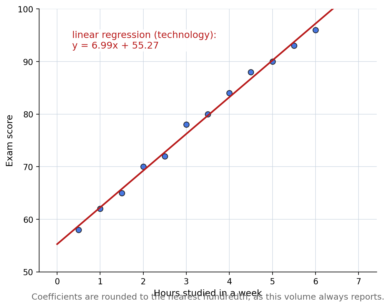
Linear model (study data):
- Strength: The points hug a straight rising trend; the line tracks the cloud.
- Weakness: The model is only about this sample and these two variables; scores cannot exceed a test's maximum even if the line eventually does; extrapolation past hours is shaky.
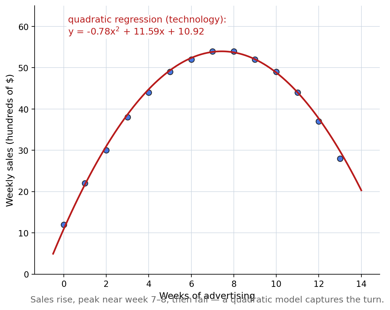
Quadratic model (advertising data):
- Strength: Captures the rise-then-fall that a line cannot.
- Weakness: Still only descriptive of this shop's weeks; a quadratic can misbehave outside the data window; it does not prove that advertising caused the sales path.
Predicting with a linear model
A.ST.1f asks you to use a linear model to predict, and to evaluate the strength and validity of the prediction, including with technology.
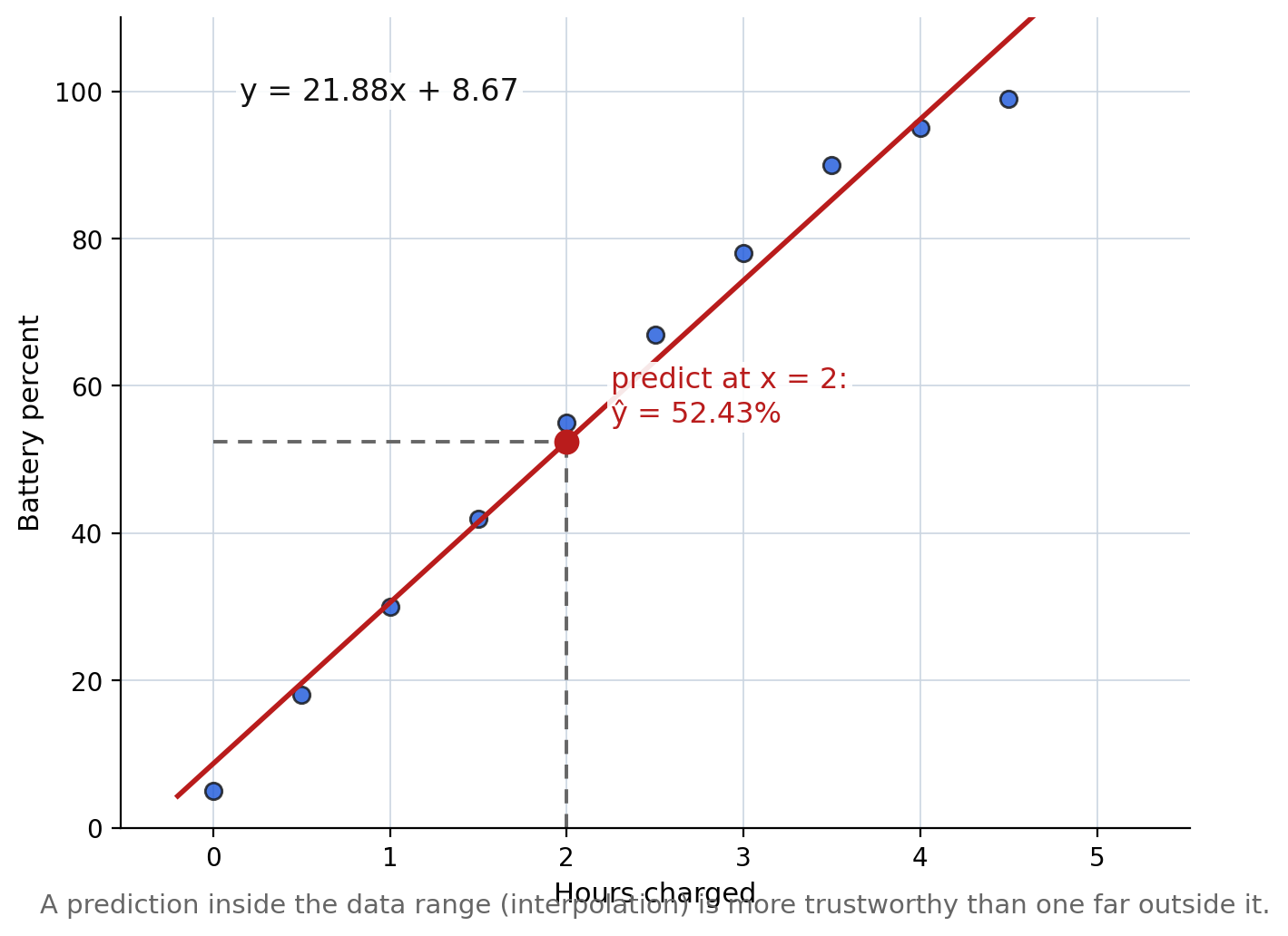
For the phone data, technology gives . At hours,
So the model predicts about battery. That sits inside the data range (interpolation) — more trustworthy than predicting at hours (extrapolation), where the line may sail past while a real battery cannot.
Technology can also evaluate for you (trace on the regression graph, table feature, or substituting in the stored equation). Either way, you judge validity: Is inside the span? Does the prediction make physical sense? Was a linear model appropriate at all?
Worked examples
Example 1 — Strength / weakness
Give one strength and one weakness of for the study data.
Answer: Strength: the scatterplot is strongly positive linear, so the line represents the relationship well inside the data. Weakness: predicting for hours of study would be extrapolation and could exceed a realistic exam maximum.
Example 2 — Predict
Using , predict battery percent after hours.
Answer: , so about .
Example 3 — Interpolation vs extrapolation
Is a prediction at for the phone data interpolation or extrapolation? At ?
Answer: is inside to — interpolation. is outside — extrapolation.
Example 4 — Invalid prediction
Using the phone model, at is . Evaluate validity.
Answer: Weak / not valid as a battery percent: it is modest extrapolation and exceeds , which a battery cannot show. Report the arithmetic, then reject or qualify the prediction in context.
Example 5 — Quadratic prediction note
A.ST.1f specifically names predictions with a linear model. If your best fit is quadratic, what is still fair to say?
Answer: You may still describe the quadratic model (A.ST.1e) and discuss what the curve suggests, but the standard's prediction bullet is about linear models — use the linear fit when you are answering A.ST.1f.
Example 6 — Technology check
How can technology help evaluate a prediction's validity beyond computing ?
Answer: Graph the residual feel (do points hug the line near that ?), compare to nearby observed -values, and visually check whether sits inside the plotted cloud.
Guided practice
- State the study-data linear model from technology.
- Give one strength and one weakness of that model.
- State the advertising quadratic model from technology.
- Using , find when .
- Is the prediction in item 69 interpolation or extrapolation? Explain.
- Why is at for the phone model not a valid battery reading?
Independent practice
Plant data linear model from technology: (days since planting, height in cm).
- Predict the height at days. Show the substitution.
- Predict at days. Classify as interpolation or extrapolation and evaluate validity.
- Give one strength and one weakness of the plant linear model.
- Using the car model , predict the value (in hundreds of dollars) of a -year-old car.
- Application. A manager uses and says weekly sales will be huge at week . Critique the claim.
- Reasoning. Explain why a model can be a good fit for the sample and still make a poor prediction for a particular new .
- Error analysis. A student computes for the study model at as , forgetting to multiply. Correct the prediction and name the mistake.
Exit ticket 19.5
- Write the phone linear model from technology.
- Predict battery percent at , and state whether the prediction is interpolation.
- Give one weakness of any regression model built from a sample.
- Why does A.ST.1f focus on linear predictions even though this chapter also teaches quadratic fits?
Lesson 19.6 — Interpreting Parameters and Communicating Conclusions
Slope and -intercept in context
A.ST.1g asks you to explain the rate of change (slope) and the -intercept (constant term) of a linear model in context.
For (hours studied, exam score):
- Slope : For each additional hour studied in a week, the model predicts about more points on the exam.
- -intercept : When (no hours studied that week), the model predicts a score of about .
Both statements need units. Both are claims about the model, not magical truths about every student.
For (car age, value in hundreds of dollars):
- Slope : Each additional year of age is associated with a predicted drop of about hundred dollars in resale value (about ).
- -intercept : At age years, the model predicts about hundred dollars. That may be an extrapolation if the data start at age — say so.
Communicating conclusions
A.ST.1i asks you to make conclusions from bivariate analysis and communicate them. A complete conclusion usually includes:
- The investigative question (or a restatement)
- The association or model you found (with the technology equation when you fit one)
- A context interpretation of key parameters (for linear models)
- The limits of the claim (sample, not causation, interpolation range)
- A clear sentence a non-classmate could understand
Worked examples
Example 1 — Slope in context
Interpret the slope of for phone charging.
Answer: Each additional hour charged is associated with about percentage points more battery, according to the model.
Example 2 — Intercept in context
Interpret the -intercept of that same model.
Answer: At hours charged, the model predicts about battery — roughly the starting charge in this sample's story.
Example 3 — Intercept may be off-data
The car model has but the youngest car in the data is year old. What caution do you add?
Answer: The intercept is a model value at , outside the observed ages — treat it as a mathematical starting value, not a measured brand-new-car price in this sample.
Example 4 — Full conclusion
Write a short conclusion for the study project.
Answer: For the Algebra 1 students in this sample, exam score and weekly study hours showed a positive linear association. Technology gave the linear model . The slope means about more points on the exam for each additional study hour, in the model. This does not prove that studying causes higher scores, and predictions are most trustworthy for study times between and hours.
Example 5 — Communicating "no model"
Conclude for the last-name data.
Answer: Among the students sampled, there was no association between letters in a last name and minutes to get to school. Neither a linear nor a quadratic curve of best fit appropriately represents the data. Last-name length is not a useful predictor of commute time in this sample.
Example 6 — Causation sentence to refuse
A headline says "Study proves more advertising causes higher sales forever." What should your communication correct?
Answer: The advertising data showed a quadratic rise-then-fall in one shop's weeks — not proof of causation, and not "forever." Past the peak, the model predicts declining sales.
Guided practice
- Interpret the slope of in context, with units.
- Interpret the -intercept of that model in context.
- Interpret the slope of in context.
- Why might the car model's -intercept need a caution?
- List three ingredients of a complete A.ST.1i conclusion.
- Rewrite as an honest conclusion: "Our scatterplot proves that studying causes better grades."
Independent practice
- Interpret both parameters of (days, plant height in cm).
- Interpret both parameters of (hours charged, battery percent).
- Application. Write a full conclusion paragraph for the car-age study, including the technology equation, parameter meanings, and a no-causation caution.
- Application. Write a full conclusion for the HVAC energy study, including why the quadratic model was chosen over the linear one.
- Reasoning. Why is "the slope is " an incomplete answer to A.ST.1g?
- Error analysis. A student interprets the slope of the car model as "the car loses per year." Correct the units.
Exit ticket 19.6
- Interpret the slope of the study model in one sentence with units.
- Interpret the -intercept of the phone model in one sentence with units.
- Give one sentence you should include whenever you communicate an observational association.
- Name the standard letter that asks you to communicate conclusions based on bivariate analysis.
Chapter 19 Review
A.ST.1a–c — Questions, variables, sampling
- Write a bivariate investigative question about temperature and lemonade sales at a school stand.
- For that question, name and .
- Describe an SRS of school days out of a -day selling season.
- Critique: surveying only rainy days, then generalizing to the whole season.
A.ST.1h — Reading scatterplots
- Describe the association in the study-time figure (positive linear / negative linear / curved / none) and justify with evidence.
- Describe the pattern in the HVAC figure and say what model type it suggests.
- Describe the last-name figure's association.
A.ST.1d–e — Technology fits and model quality
- State the study linear model from technology.
- State the HVAC quadratic model from technology, and give one reason it beats the linear fit .
- State the advertising quadratic model from technology.
- Give one strength and one weakness of the study linear model.
A.ST.1f–g — Predict and interpret
- Using , predict battery percent at . Is it interpolation?
- Using , predict the exam score at .
- Using , discuss validity of a prediction at .
- Interpret the slope and -intercept of in context.
- Interpret the slope and -intercept of in context.
A.ST.1i — Communicate
- Write a four-sentence conclusion for the phone-charging study.
- Write a four-sentence conclusion for the last-name study (no appropriate linear/quadratic model).
Mixed applications
- Application. A data set has pairs showing a clear positive linear trend. Outline the technology steps to obtain and record the curve of best fit.
- Application. A data set has pairs in a U-shape. Explain how you would use technology to choose between linear and quadratic.
- Reasoning. Why does this chapter refuse calculator-free regression?
- Error analysis. A student reports "because it was easier than the calculator's ." What did the student violate?
Cumulative performance
- For the plant data, state the technology linear model , predict height at day , and interpret slope and intercept.
- For the car data, state , predict at age , and write a no-causation caution.
- For the HVAC data, give both technology equations (linear and quadratic) and state which you report as the curve of best fit.
- Formulate a new bivariate question that the advertising result raises, naming variables for a follow-up cycle.
Standards coverage check — Chapter 19
| Knowledge and Skill | Aspect | Where it is taught | Where it is practiced | Where it is interpreted in context |
|---|---|---|---|---|
| A.ST.1a — formulate bivariate investigative questions | Question design | 19.1 | 1–16; 99 | 10, 14, 99, 124 |
| A.ST.1b — determine variables | Independent / dependent choice | 19.2 | 17, 18, 23, 28–29; 100 | 23, 25, 100 |
| A.ST.1c — representative sample, including SRS | Sampling methods | 19.2 (fig2) | 19–22, 24–27, 30–32; 101, 102 | 25, 101 |
| A.ST.1d — technology chooses linear vs quadratic; ≤30 points; equation | Fit choice with technology | 19.4 (fig7, fig8) | 50–65; 106–108, 117, 118, 123 | 59, 123 |
| A.ST.1e — regression via technology; strengths and weaknesses | Model write-up | 19.5 (fig9, fig10) | 66–68, 74, 76; 109 | 67, 74, 109 |
| A.ST.1f — predict with linear model; evaluate validity | Predictions | 19.5 (fig11) | 69–73, 75, 77–82; 110–112 | 71, 73, 76, 112 |
| A.ST.1g — interpret slope and -intercept in context | Parameter meaning | 19.6 | 83–86, 89–90, 93–96; 113, 114, 121 | 83–86, 89–94, 113, 114, 121 |
| A.ST.1h — analyze relationships in a scatterplot | Pattern reading | 19.3 (fig3–fig6) | 33–49; 103–105 | 38, 42, 47 |
| A.ST.1i — conclusions and communication | Report results | 19.6 | 87–88, 91–92, 97–98; 115, 116, 124 | 91, 92, 115, 116 |
Supporting items: 3, 6, 8, 11–12, 39–40, 44–45, 56, 60–61, 119–120 fix process habits — pairing, the cycle's return, the 30-point limit, and the ban on calculator-free "regression."
Boundaries respected. Every regression set has ≤30 points. Curves of best fit are linear or quadratic and always attributed to technology. Predictions under A.ST.1f use linear models. Correlation coefficients are never required as answers. Association is not causation appears wherever conclusions are communicated.
Answer keys for every item in this chapter are in Appendix A.